In production AI, models rarely fail catastrophically. They degrade. Quietly. A credit risk model trained in a low-rate environment begins misclassifying borrowers few months after rates double. An inference pipeline silently drops a third of its records due to an upstream schema change, and no one notices until a compliance review surfaces the anomaly. By then, decisions have already been made on corrupted signals.
In regulated industries, financial services in particular, where credit risk models must conform to model risk management guidelines, this is not a technical inconvenience but a regulatory exposure.
Databricks has natively solved this problem by evolving Lakehouse Monitoring into a fully integrated, Unity Catalog-governed suite: Data Quality Monitoring. This is not a monitoring add-on. It is an architectural component of the platform, designed so that observability is embedded, not bolted on afterward.
The Architecture: Two Complementary Pillars
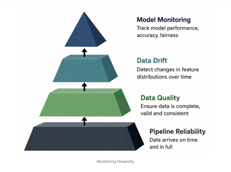
The most common mistake in ML observability is treating data quality and the drift as the same problem. They are not. Before we can ask whether feature distributions have shifted, we must first verify that the data arrived on time and at the right volume.
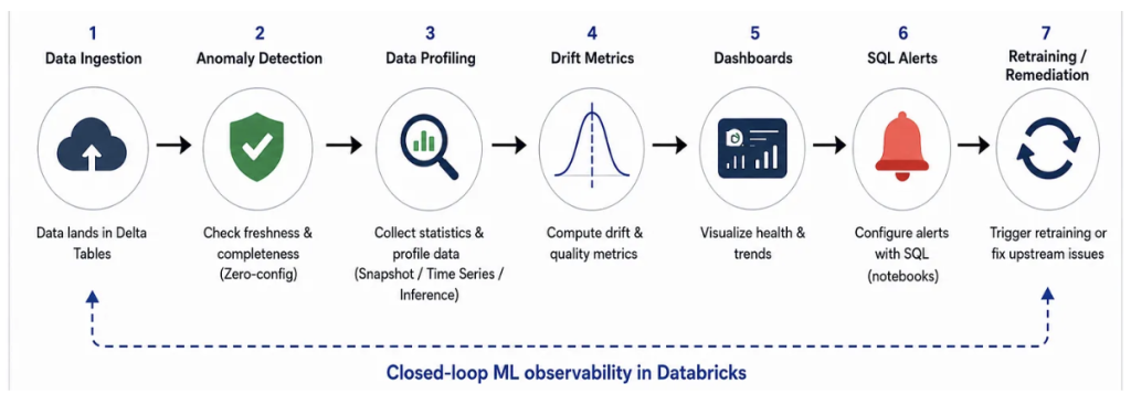
Databricks addresses this by decomposing observability into two distinct, native capabilities:
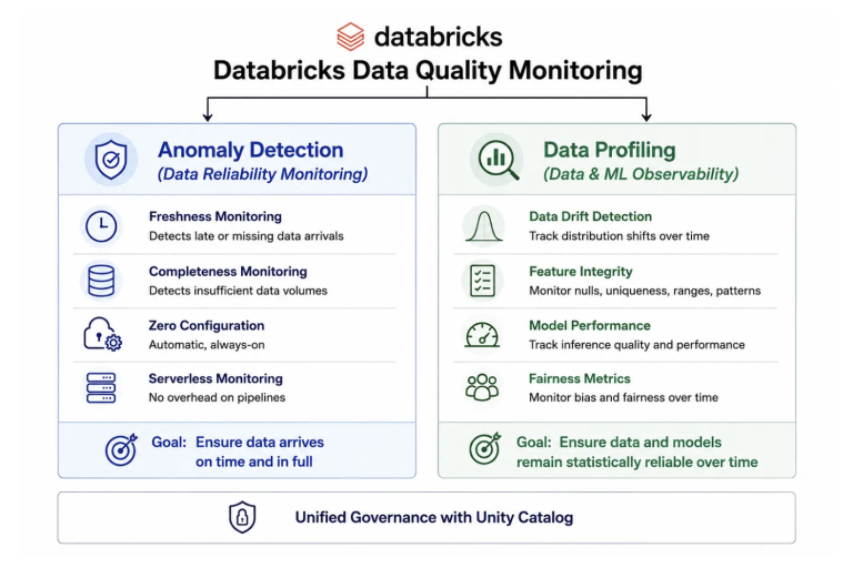
Anomaly Detection: Monitoring for data reliability. Schema-level, zero-configuration monitoring that ensures data is arriving and arriving correctly before any statistical analysis begins.
Data Profiling: Observability for data and ML. Table-level statistical monitoring that tracks distribution shifts, feature integrity, and model performance over time. Formerly known as Lakehouse Monitoring.
Both capabilities live inside Unity Catalog. Confusing between them leads to monitoring architectures that catch the drift while missing the silent pipeline failure that invalidated the batch upstream.
Pillar 1: Anomaly Detection
Anomaly Detection is enabled at the schema level. Navigate to any schema in Catalog Explorer, open the Details tab, click enable the Data Quality Monitoring dialog, turn on Anomaly detection, then click Save. Databricks handles the rest.
Freshness and Completeness
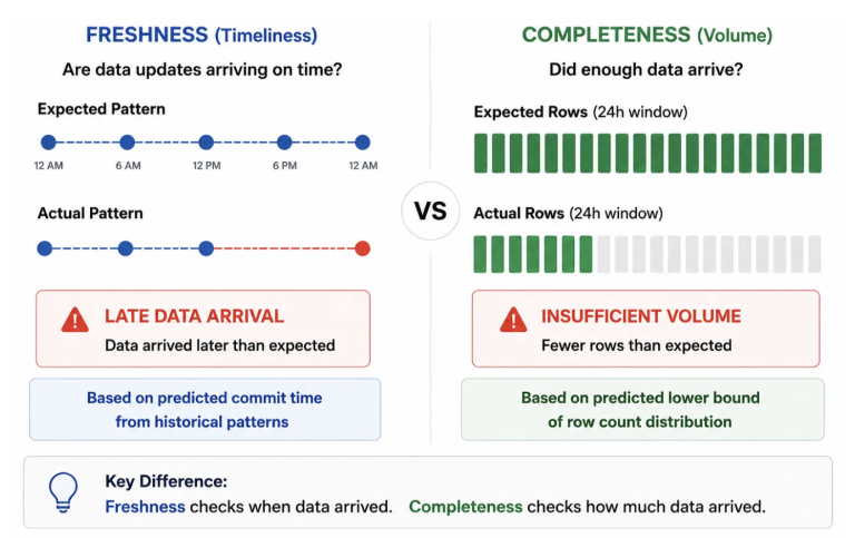
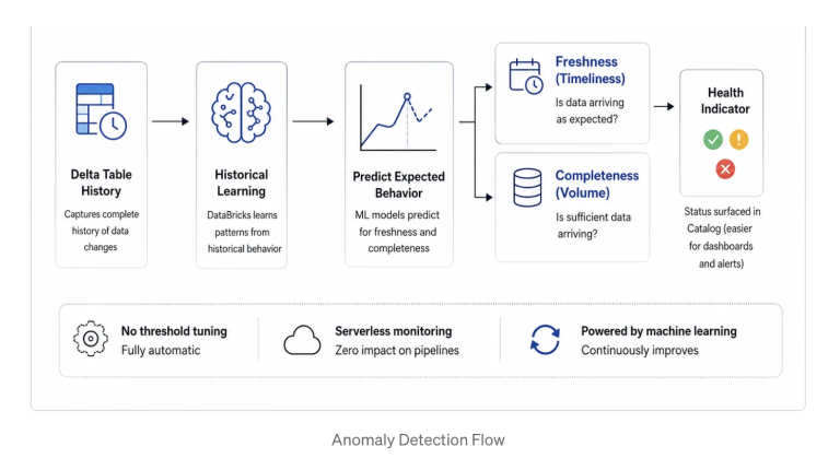
Freshness measures how recently a table was updated. Databricks builds a per-table predictive model from the historical pattern of Delta commits. If a commit arrives significantly later than expected because an upstream job failed, or a dependency timed out then the table is flagged as stale. No threshold tuning is required. The model learns the expected delivery cadence from history, and deviation from that cadence becomes the signal.
Completeness measures row volume. Databricks analyzes the historical distribution of rows written to the table within any 24-hour window and establishes a predictive lower bound. If overnight batch volume falls below this lower bound, the table is marked as incomplete. This is specifically about whether sufficient data arrived.
Percent null adds a column-level completeness check (beta as of June 2026). Databricks predicts an expected range for nulls over the last 24 hours, and if a column’s percent null exceeds the upper bound, that table is also marked incomplete.
A critical operational point: Anomaly Detection runs on serverless compute and adds zero overhead to the pipelines populating your tables. It observes passively.
Intelligent Scanning
Databricks does not scan every table at the same frequency. The intelligent scanning engine prioritizes tables by downstream usage and popularity for example, the number of queries, dashboards, and downstream tables that depend on each one. High-impact tables are evaluated most aggressively. Low-impact tables are scanned less frequently. Critical data assets receive the most monitoring attention automatically, without manual prioritization.
Tables can be explicitly excluded from scanning using the `excluded_table_full_names` parameter in the Create or Update Monitor API.
One planning consideration: smart scanning may delay the population of health indicators by up to two weeks for tables skipped during the initial scan. The indicator is populated at the next scheduled rescan. Account for this window when rolling out monitoring across a new schema.
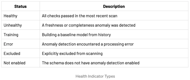
Health Indicators and the Catalog Explorer Surface
Once a scan completes, health indicators appear on table and schema pages in Catalog Explorer. Any user with `SELECT` or `BROWSE` permission can see the health status of a table without navigating to the Data Quality Monitoring UI. This surfaces data reliability directly in the environment where data consumers already work.
Incident Management
Unhealthy tables surface in the Unhealthy tab of the Data Quality Monitoring UI with the reason (freshness or completeness), first detection timestamp, root cause analysis, and a downstream impact classification (High, Medium, or Low) based on the number of dependent tables and queries.
From the incident details view, two resolution actions are available:
Assign to me: Claims ownership of the incident to indicate active investigation. The table remains Unhealthy. The assignment persists for seven days.
Not an issue: Marks the incident as a false positive and dismisses it. The table reverts to Healthy, and the resolution is logged in the Recently Resolved Incidents section. The dismissal also persists for seven days.
The auto-resolved incidents view deserves equal attention. These are self-healing issues such as upstream delays or staleness windows that resolved once fresh data arrived. Reviewing them over time separates flaky pipelines from persistent structural problems and provides evidence of transient issues for compliance documentation.
Programmatic Alerting: The System Table
All anomaly detection results are written to `system.data_quality_monitoring.table_results`, a system table accessible across the entire metastore. This table can be queried directly in Databricks SQL to build custom alerts, filtered by catalog, status, and scan timestamp. By default, only account admins have access to it. If your MLOps team needs to configure alerts or automated responses against it, explicit `GRANT` statements are required before any automation is built on top of it.
Pillar 2: Data Profiling
Where Anomaly Detection verifies that the pipeline is flowing, Data Profiling verifies that the data means what it is supposed to mean. For ML teams, this is where the operational signal lives.
Profile Types
Data Profiling supports three profile types. Choosing the right one depends on whether your table has a time dimension and whether it contains model prediction data.
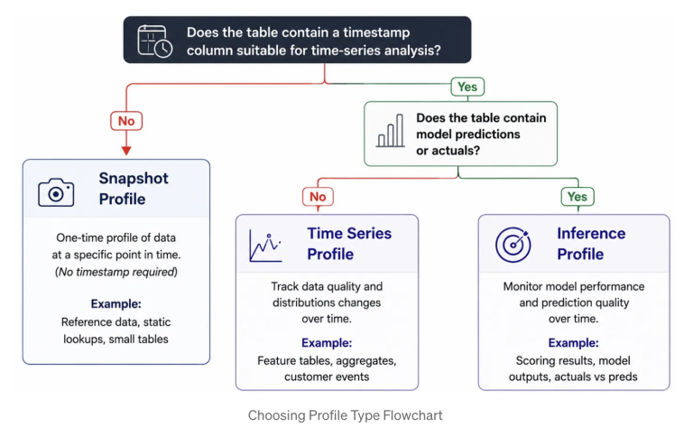
1. Snapshot profile works against any Delta managed table, external table, view, materialized view, or streaming table, with no timestamp column required. Every refresh re-processes the entire table and CDF does not apply. This makes Snapshot appropriate for tables that are relatively static or updated infrequently: reference data, configuration tables, dimension tables, or any table where a current-state quality assessment is more valuable than trend analysis. The maximum supported table size is 4TB and for tables larger than this, a Time Series profile is the recommended alternative.
2. Time Series profile is for tables that have a meaningful timestamp column and where understanding how data properties change over time windows is the primary concern. Profiling partitions data into configurable time windows with granularities from 5 minutes to 1 year and computes quality metrics over time, enabling trend detection and window-to-window drift comparison. The timestamp column must be of TIMESTAMP type, or a type convertible using the `to_timestamp` function. Use Time Series for event streams, feature tables with event timestamps, and any dataset where detecting distribution shifts over a rolling window matters more than a single point-in-time view. CDF is strongly recommended: with it enabled, each refresh processes only newly appended rows rather than re-scanning the full table. Note that profiles defined on materialized views do not support incremental processing regardless of CDF.
3. Inference profile is similar to Time Series profile, additionally it also has model quality metrics. This profile is used to track the performance of machine learning models and model-serving endpoints by profiling inference tables. These profiles are specifically designed for tables that store machine learning model request logs, with one row per inference request and its prediction. The tables include columns for a timestamp, a model ID, model inputs, predictions, and optionally ground truth labels for both classification and regression models. The profile compares model performance and data quality metrics across time-based windows.
Tables for Inference profiles also support demographic metadata columns that are not used as inputs to the model but are useful for fairness and bias analysis. This capability is directly relevant in regulated domains where disparate impact must be documented and audited.
Change Data Feed (CDF) is strongly recommended for the same efficiency reasons as with Time Series profiles.
A practical decision rule: if the table has no timestamp, use Snapshot. If it has a timestamp and contains feature or event data, use Time Series. If it has a timestamp and contains model predictions, use Inference.
The 30-Day Lookback
This is the implementation nuance and most teams discover only after a painful production deployment.
When you first create a Time Series or Inference profile, Databricks processes only the data from the last 30 days prior to creation. Any older data in the table is ignored. After the monitor is created, all newly appended data is processed on each refresh. The consequence: if you attach a monitor to a table that already contains six months of inference history, only the most recent 30 days of that history will ever be evaluated. The good news is, Databricks account team helps in adjusting this 30 day limit.
Since all the newly added data will be processed after creating these profiles, enabling CDF is strongly recommended for both Time Series and Inference profiles. When active, each refresh processes only newly appended rows rather than re-scanning the entire table. As inference logs grow to hundreds of millions of rows, this is the difference between a two-minute refresh and a two-hour one.
Primary Table and Baseline Table
A table that is to be profiled is called Primary Table. In addition to the primary table being profiled, you can optionally specify a baseline table as a reference for measuring drift that is, the change in values over time. The baseline table should contain data that reflects the expected statistical distributions, column distributions, missing value rates, and overall data quality characteristics of the input data. It must match the schema of the primary table, with the exception of the timestamp column for Time Series and Inference profiles.
The appropriate baseline varies by profile type. For Snapshot profiles, use a prior snapshot where distributions represent an acceptable quality standard. For Time Series profiles, use data from time windows where distributions were within expected norms. For Inference profiles, the ideal baseline is the training or validation dataset. Drift is then measured relative to what the model was actually trained on, and the baseline must include the same feature columns and the same `model_id_col` as the primary table to ensure consistent aggregation.
Output Tables: Profile Metrics and Drift Metrics
Every profile generation produces or updates two output Delta tables:
1. Profile Metrics contains per-column, per-time-window statistics: row counts, means, null/zero percentages, distinct value counts and quantile distributions. For Inference profiles, it also includes model performance metrics (such as accuracy, precision, recall, F1, confusion matrix, RMSE, MAPE, R²) plus fairness and bias metrics.
2. Drift Metrics contains statistics related to the data’s drift over time. The drift table is generated or updated when a baseline table is provided or when a consecutive time window exists after aggregation. The two types of drift computed are:
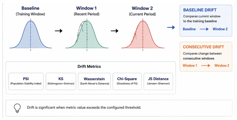
BASELINE: Compares each time window against the baseline table distribution. Detects gradual regime drift that accumulates over weeks or months and is invisible to consecutive-only monitoring.
CONSECUTIVE: Compares each time window against the immediately preceding window. Detects abrupt changes such as feature pipeline regressions, data source migrations, or upstream schema changes.
For each column, Databricks applies statistically appropriate tests based on data type. For numerical columns: the Kolmogorov-Smirnov (KS) test, Wasserstein distance, and Population Stability Index (PSI). And, for categorical columns: Chi-squared test, Total Variation (TV) distance, L-infinity distance, and Jensen–Shannon (JS) distance.
Additionally, the drift metrics table carries `count_delta`, `avg_delta`, `percent_null_delta`, `percent_zeros_delta`, and `percent_distinct_delta` giving a complete quantitative picture of the shift between windows.
The Monitoring Dashboard
When a profile runs, Databricks automatically generates a dashboard displaying key metrics computed by the profile. The visualizations included depend on the profile type with different metrics organized into sections. The dashboard is created in the user’s account and is customizable and shareable like any other dashboard. Teams can modify existing charts, add new ones, and adjust user-editable parameters for date range, data slices, and model filters across the entire dashboard or for individual charts.
Use Case: Credit Risk Monitoring on the Lakehouse
Business Problem
A financial institution wants to operationalize a credit risk model in production, but the real challenge is not just model training. It is proving that incoming data remains timely, complete, statistically stable, and operationally trustworthy as macroeconomic conditions change.
The business problem is therefore two-fold: protect the upstream data pipeline from hidden failures, and detect when the model is making decisions on data that no longer resembles the environment it was trained on. In regulated settings, that monitoring layer must also create an auditable record for investigation, escalation, retraining, and governance review.
Data
The use case is built on synthetic borrower application data designed to simulate realistic economic regime changes across stable, stressed, and recessionary periods. The dataset includes core underwriting features such as annual income, debt-to-income ratio, loan amount, interest rate, credit score, employment length, number of open accounts, recent delinquencies, home ownership, and loan purpose.
The target label is a credit risk grade, represented as ordered classes from A through E. Because the data is synthetic, the use case is safe for demonstration while still being rich enough to show how input drift, data quality degradation, and model performance decay emerge together in a production-like environment.
Medallion Architecture
A Medallion architecture provides the right operating model for this use case. The Bronze layer captures raw loan application events exactly as they arrive from source systems, preserving lineage and making it possible to apply freshness and completeness monitoring at the point of ingestio
The Silver layer standardizes and validates the records, applies data quality checks, resolves schema issues, and prepares consistent business-ready fields for downstream consumption. The Gold layer produces model-ready features and the inference log used for quality monitoring, making it the right place to evaluate drift, feature integrity, and outcome quality over time.
Model Development and Management with MLflow
The model development flow follows a standard Databricks MLOps pattern. A classification model is trained on a stable historical window, feature engineering is versioned in the pipeline, and experiments are tracked in MLflow so that parameters, metrics, model artifacts, and validation outcomes are captured in a reproducible system of record.
Once validated, the model is registered for governed deployment and promoted through the model registry. This creates the operational baseline for monitoring: the production model, its training window, and its evaluation results become the reference point against which future production behaviour can be compared.
Monitoring
Once deployed, Data Quality Monitoring becomes the control plane for the end-to-end use case. At the data layer, anomaly detection protects the ingestion and transformation pipeline by flagging delayed arrivals and unexpected drops in volume. At the model layer, data profiling on the inference log tracks how feature distributions, prediction behavior, and model quality evolve across time-based windows.
The dashboard turns those metrics into an operational workspace. For this use case, the most valuable sections are Model Performance, Feature Profiling, Drift Analysis, Data Quality, Fairness and Bias and Inference Volume. Together, they show whether accuracy, precision, recall, and F1 are degrading; which numerical or categorical features are drifting; where null, zero, or invalid value issues are emerging; whether fairness metrics are changing across demographic slices; and whether the scoring volume itself has shifted enough to explain or intensify the observed behavior.
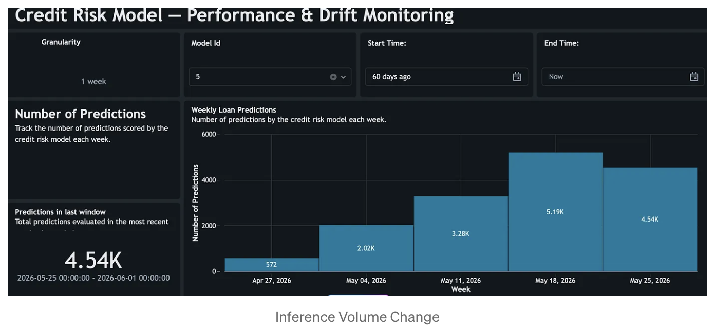
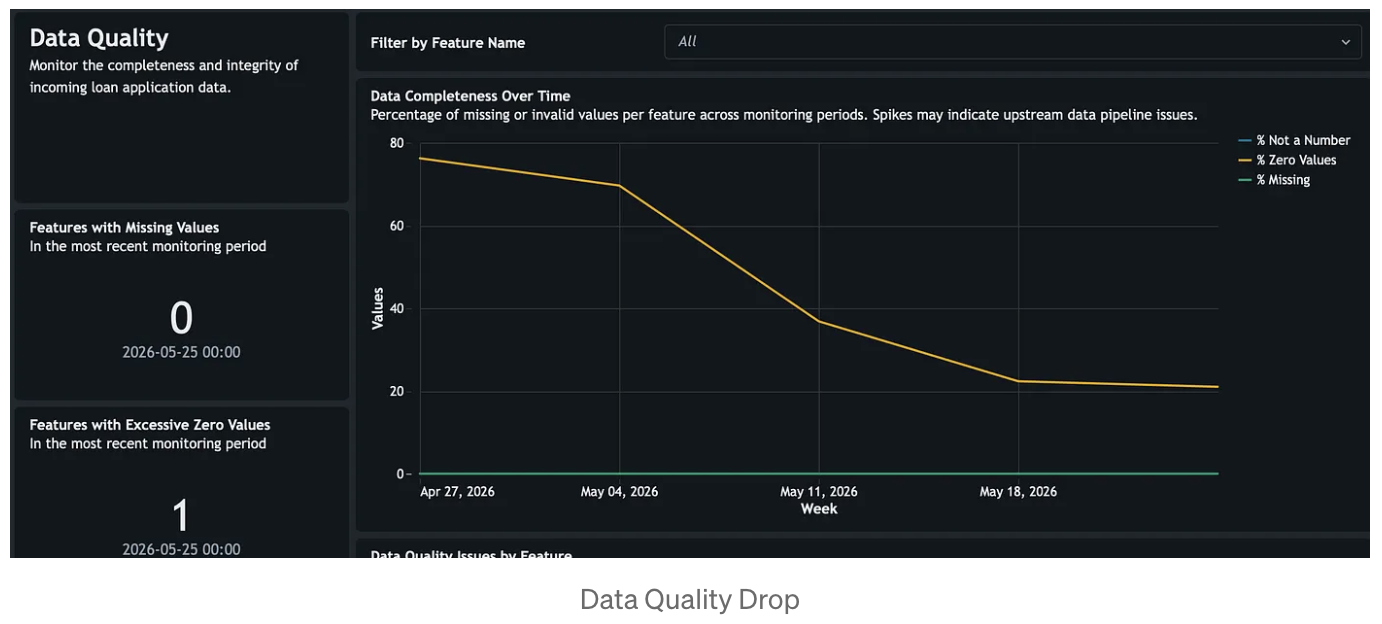
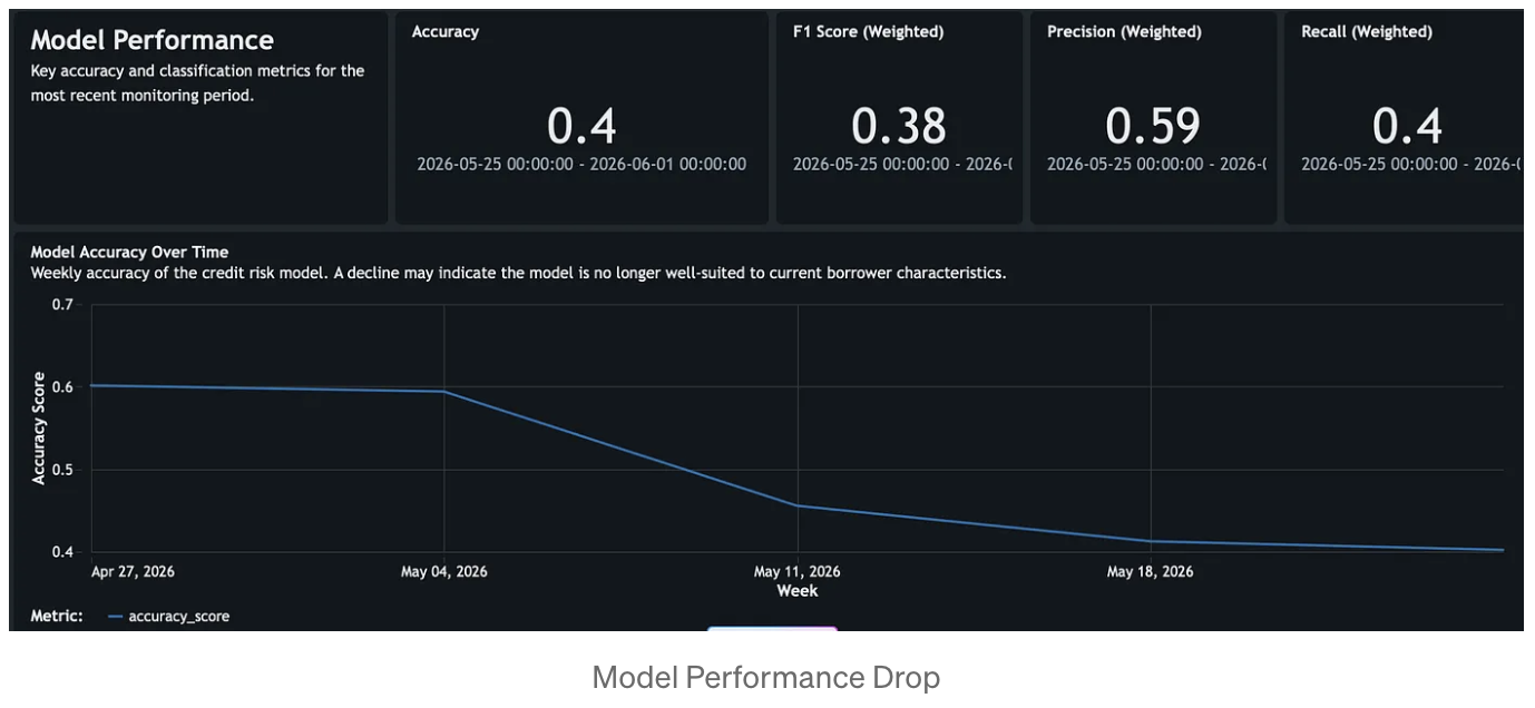
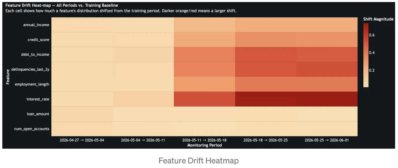
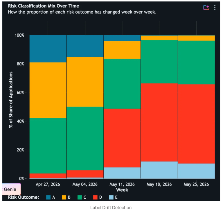
In the credit risk scenario, this monitoring pattern makes deterioration visible early. A model trained in a stable economy can still appear operational while silently drifting out of policy relevance as rates rise, borrower quality changes, and delinquency patterns worsen. By combining baseline drift, consecutive drift, performance metrics, and data quality indicators in one view, the monitoring system tells a coherent story about what changed, when it changed, and where to investigate first.
Closing the Loop: From Observation to Automated Action
Monitoring without action is expensive logging. The operational architecture must close the feedback loop: observation triggers retraining, retraining restores performance, and the cycle repeats.
A Databricks SQL Alert configured against the Drift Metrics output table serving as the trigger. The alert queries the baseline drift rows for features where KS test p-values fall below a significance threshold, with annual income, debt-to-income ratio, and interest rate acting as high-priority signals in a credit risk context. When the alert trips, it fires a webhook notification that triggers a Databricks Job. That job pulls the most recent feature data from the Gold layer, retrains the model via MLflow with a fresh training window, evaluates it against a holdout set, and registers a new champion version in the model registry. The production serving endpoint then picks up the new version, and the monitoring cycle restarts.
This architecture satisfies the core governance requirement behind modern model risk management. The Drift Metrics table becomes the evidence trail, capturing when drift was detected and what triggered the response. MLflow captures every retraining run, hyperparameter choice, and evaluation result. Unity Catalog lineage connects the model version back to the data and transformation pipeline that produced it. The result is not just automated retraining, but automated retraining with traceability, reproducibility, and auditability.
Conclusion
The failure mode of production ML is not a model that stops working overnight. It is a model that degrades slowly, on data that drifts silently, in a pipeline no one is watching. By the time the signal surfaces in business metrics, the damage is done.
Databricks Data Quality Monitoring closes this gap architecturally. Anomaly Detection protects the pipeline, ensuring data arrives on schedule and at the right volume, flagging failures before they reach inference. Data Profiling interrogates the data, tracking statistical distributions, feature integrity, model performance, and fairness across every time window. The monitoring dashboard surfaces all of this through a production-ready analytical interface. And SQL alerts against the drift metrics output tables convert passive observation into active automated remediation.
The patterns covered here Anomaly Detection, CDF enabled profiles, dual consecutive and baseline drift tracking, triaged data quality monitoring, fairness/bias metrics integration and SQL alert-triggered retraining form a reproducible blueprint for any team operating ML models in a regulated or high-stakes environment.
Build systems that know when they are failing. Build systems that know how to heal themselves. Databricks Data Quality Monitoring enables it.